
by Miguel Posada
This work was done by LaGuardia student Miguel Posada as a part of the Honors “General Physics I” class, Fall 2023. In this work, Miguel investigates the Maupertuis's principle in classical mechanics and establishes its correspondence to the variational principle in quantum mechanics.
The research was conducted under the supervision of Dr. Roman Senkov.
Other research projects done by students in the Physics Honors courses: “Orbital Decay of a Massive Black Hole”, “Atomic Nuclei and Pairing Correlations”, “Computer Modelling of Physical Systems”, “Lagrange Points in Binary Star Systems”, and “Unveiling Stellar Dimensions: An Exploration of Neutron Stars and White Dwarfs”.
Download this article: pdf (700Kb)
In classical mechanics, Maupertuis's principle is used to determine the trajectories of a set of particle, it is a simplified form of the principle of least action [1,2]. Instead of solving the standard equations of motion, Maupertuis's principle enables the determination of an object's actual path by optimizing its mechanical energy, with the condition that the area outlined by the object's trajectory in the phase-space diagram remains constant. This principle offers a unique perspective on the origin of the well-known variational principle in quantum mechanics [3,4], when, instead of directly solving the Schrödinger equation, the system's energy is minimized. In this work, we apply Maupertuis's principle to the two simplest systems in classical mechanics: motion under a constant force and simple harmonic motion. We then establish the correspondence between Maupertuis's principle and the variational principle in quantum mechanics. By highlighting the similarity between these two principles, our work demonstrates a non-trivial internal connection between the quantum and classical realms.
In his attempt to understand behavior of macroscopic objects, Sir Isaac Newton developed a set of equations and principles that are known as Newton's laws of motion [1,5]. For example, according to the second Newton's law, assuming that the motion is described in an inertial frame of reference, a particle moving in a force field acquires the following acceleration \begin{equation}\tag{1} a = \frac{F}{m}, \end{equation} where \(m\) is the particle's mass and \(F\) is the net external force acting on the particle.
While Newton's laws of motion have been successfully implemented on the macroscopic scale, the subatomic realm requires a significantly different and more complicated approach, one that is based on the Schrödinger equation and principles of quantum mechanics [3,4]. Stationary Schrödinger equation in 1-D can be written as \begin{equation}\tag{2} E \psi = - \frac{\hbar^2}{2m} \frac{\partial^2 \psi}{\partial x^2} + U(x) \psi, \end{equation} here \(\psi(x)\) is the wavefunction of the system, \(x\) is the particle's position, \(U(x)\) is the potential energy and \(E\) is the total mechanical energy of the system, and \(\hbar\) is the reduced Planck constant.
Looking at Eqs.(1,2) it may not be obvious, however quantum mechanics is closely related to and takes its origin from classical mechanics. An example of this relationship is found in the quasi-classical approximation, where, in the limit of large quantum numbers, solution of the Schrödinger equation (2) converges towards the classical trajectories given by Eq.(1). This approximation not only demonstrates how classical mechanics can be viewed as a special case within the broader quantum framework but also highlights the seamless transition from the classical to the quantum world.
Another example of such a relationship is Maupertuis's principle in classical mechanics and the variational principle in quantum mechanics. In both approaches, to find the actual trajectory, the average energy of the system is minimized under certain very specific conditions: \begin{equation}\tag{3} E(\mbox{“actual trajectory”}) = E_{min}. \end{equation}
Let us restrict our consideration only to bound states when the motion is finite and repeats. In this case, in the classical approach, the condition is that the area in the phase-space diagram outlined by the object's trajectory should remain constant \begin{equation}\tag{4} W = \oint p dx = \mbox{const}, \end{equation} where \(W\) is the area under the curve \(p=p(x)\), \(p=mv\) is the momentum and \(x\) is the position of the particle. The restriction that the motion repeats itself helps to define integration (4) and simplify the consideration.
In the quantum approach, the minimization occurs for fixed quantum numbers \(n\), and, according to the Bohr-Sommerfeld quantization rule [6,7], fixed quantum numbers correspond to fixed areas in the same phase-space diagram \begin{equation}\tag{5} W = \oint p dx = 2 \pi \hbar n, \end{equation} where \(\hbar\) is the reduced Planck constant and \(n\) is the quantum number.
Thus, both principles correspond perfectly to each other. While the variational principle is well-known and widely used for real calculations in quantum mechanics, Maupertuis's principle is less practical and has mostly theoretical interest.
More specifically, in this work, we aim to understand how Maupertuis's principle works and apply it to two simple classical systems such as motion of a particle in a constant force fields and simple harmonic motion. We will also demonstrate the correspondence of Maupertuis's principle to the variational principle in quantum mechanics, which can serve as a testament to the underlying unity of the physical laws governing the universe, bridging the gap between the microscopic and macroscopic domains.
Pierre Louis Maupertuis introduced his principle aiming to determine the trajectory of an object or particle by optimizing a certain functional (a function of the trajectory). In this work, we consider an unusual version of Maupertuis's principle, which requires the minimization of the particle's average mechanical energy.
To apply this version of the Maupertuis's Principle, first, we need to describe the trajectory of our system using the so-called phase-space diagram: for one degree of freedom, it is a two-dimensional plane with momentum or velocity as the y-axis and position as the x-axis. Thus, each point on the phase-space diagram corresponds to a certain position and velocity of the particle and completely describes the state of the system.
Furthermore, for a given trajectory, we can determine the system's average mechanical energy, which is the sum of its kinetic and potential energies, and calculate the area in the phase-space diagram outlined by the trajectory (assuming that motion repeats itself and the system comes to its initial position after some time \(T\)).
Finally, by varying the trajectory, we can obtain different values for the energy and area. Maupertuis's principle states that the actual trajectory delivers a minimum to the energy under the condition that the area in the phase-space diagram remains constant. Thus, by minimizing the average energy, we can determine the actual trajectory of the system. The following are two examples of the application of this principle.
Let's consider a periodic motion of an object under action of a constant force and a rigid floor: at \(t=0\) the object is at the ground, \(x=0\), and has positive initial velocity \(v_0\) pointing up; then the object travels up and slows down until it comes to a complete stop at \(x=L\) (let's take that the force points down and does not allow the object to fly away); then the object starts moving down towards the ground, and, after an elastic collision with the ground, the motion repeats starting with the same initial velocity \(v_0\), see Fig. 1.
The described motion can be parameterized as a function of time \(t\) as \begin{equation} \tag{6} \left\{ \begin{array}{ll} x = v_0 t- \frac{at^2}{2}, & \text{position as a function of time} \\ v = v_0 - at, & \text{velocity as a function of time} \end{array} \right., \end{equation} where \(v_0\) is the object's velocity at the ground, and \(a\) is the acceleration. Here we assumed constant acceleration motion and treat the acceleration and the initial velocity as free parameters. Note: we do not know the value of the acceleration since we do not assume any Newton's laws.
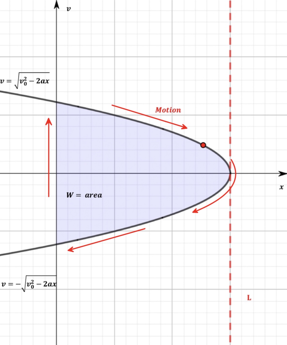
Figure 1: Phase-space diagram for motion under constant force.
Calculating the area under the trajectory. Considering the one-dimensional motion (6) we can eliminate time and find velocity as a function of position \begin{equation}\tag{7} v = \pm \sqrt{v^2_0-2ax}, \end{equation} where the signs corresponds to: '+' is for motion up and '-' for motion down.
Analyzing the motion of the particle and limiting the position \(x\) between the ground (\(x=0\)) and the maximum position (\(x=L\)), we can compute the area on the phase-space diagram (see Fig. 1, the shaded part) as follows: \begin{equation}\tag{8} W = 2\int_{0}^{L} v \, dx = 2 \int_{0}^{L} \sqrt{v^2_0-2ax} \, dx = \frac{2v^3_0}{3a}, \end{equation} where the mass multiplier was omitted (\(m\)=constant), the factor 2 is due to areas above and below the \(x\)-axis, and the maximum position \(L\) is the position where the particle momentarily stops: \begin{equation}\tag{9} \sqrt{v^2_0-2aL} = 0 \, \rightarrow L = \frac{v_0^2}{2a}. \end{equation} Using the maximum position (9) eliminates the contribution from the upper limit in integration (8).
Calculating average mechanical energy. Mechanical energy is the sum of a system's kinetic and potential energies: \(E = KE + U\). Let us first consider kinetic energy. We need to calculate the ball's average kinetic energy, which can be defined as an integration over the time evaluated from time zero to the period divided by this period \begin{equation}\tag{10} \langle KE \rangle = \frac{1}{T} \int_0^T\frac{1}{2}mv^2 dt, \end{equation} here \(\langle...\rangle\) means average over time, \(m\) represents mass, \(v\) represents speed, and \(T\) is the period of the motion. Using \(v=v_0-at\) from Eq.(6), we can write \begin{equation}\tag{11} \langle KE \rangle = \frac{m}{2T}\int_{0}^{T}(v_0-at)^2dt = \frac{m}{2T}\left(v_0^2 T - v_0aT^2 + \frac{1}{3} a^2T^3\right). \end{equation} After substituting \(T=v_0/a\) and simplifying the integral, the resultant average kinetic energy for the particle's motion becomes \begin{equation}\tag{12} \langle KE \rangle =\frac{mv^2_0}{6}. \end{equation}
Halfway through the computation of mechanical energy, the only missing constituent is the potential energy that for a constant force can be written as \begin{equation}\tag{13} U = - Fx, \end{equation} where \(F\) is the force, the position \(x\) as a function of time is defined by Eq.(6), thus, the average position can be found as follows, \begin{equation}\tag{14} \langle x \rangle =\frac{1}{T}\int_{0}^{T}xdt = \frac{1}{T}\int_{0}^{T}\left(v_0 t- \frac{at^2}{2}\right)dt = \frac{1}{T} \left( \frac{v_0 T^2}{2} -\frac{aT^3}{6}\right). \end{equation} After further simplification involving \(T={v_0}/{a}\), the average position is: \begin{equation}\tag{15} \langle x \rangle = \frac{v^2_0}{2a}-\frac{v^2_0}{6a}=\frac{v^2_0}{3a}. \end{equation}
Using the result of integration (15) and the definition (13) the average potential energy equals to \begin{equation}\tag{16} \langle U \rangle = -F\frac{v^2_0}{3a} = |F|\frac{v^2_0}{3a}. \end{equation} In this case, the force F is negative (we need a returning force bringing the object back to the ground), so it is convenient to represent the force as \(F=-|F|\). Now that we have kinetic \(\langle KE \rangle\) and potential \(\langle U \rangle\) energies, we can set up the equation for the average mechanical energy \begin{equation}\tag{17} \langle E \rangle=\frac{mv^2_0}{6} + |F|\frac{v^2_0}{3a}. \end{equation}
Optimization of energy. Now that the first two steps of Maupertuis' principle have been established, we can vary the trajectory maintaining the area constant (see Fig. 2) and trying to minimize the energy (17).
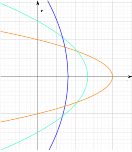
Figure 2: Variations in parameters \(v_0\) and \(a\) while maintaining the area \(W\) constant.
We can use the area equation (8) to isolate acceleration and replace it in the mechanical energy equation. \begin{equation}\tag{18} W=\frac{2v^3_0}{3a}\rightarrow a=\frac{2v^3_0}{3W}. \end{equation} \begin{equation}\tag{19} \langle E \rangle=\frac{mv^2_0}{6} + |F|\frac{v^2_0}{3a} = \frac{mv^2_0}{6}+\frac{|F|W}{2v_0}. \end{equation} Finally, by using the average mechanical energy equation and optimizing it, we can determine the minima extremum, which will correspond to the lowest energy state for the system while maintaining a constant area.
The first derivative of the energy with respect to the initial velocity is: \begin{equation}\tag{20} \frac{d\langle E\rangle}{dv_0}=\frac{mv_0}{3}-\frac{|F|W}{2v_0^2}=0 \end{equation} and \begin{equation}\tag{21} v_0^3 = \frac{3|F|W}{2m} \mbox{ and } a = \frac{2v^3_0}{3W}, \end{equation} or \begin{equation}\tag{22} a = \frac{F}{m}. \end{equation} We did not assume any value for the acceleration \(a\), formula (22) came out as a result of the minimization. Thus, optimizing mechanical energy while maintaining the area constant results in Newton's second law of motion. This means the actual trajectory the object undergoes is when the object's acceleration equals to the force over the mass. This was derived from the Mauperuis's principle.
Let's consider an ideal harmonic oscillator, where a spring is fixed on one side and on the other side is attached to an object with mass \(m\). The spring is later compressed and released, so the mass undergoes SHM, which can be parameterized as \begin{equation}\tag{23} \left\{ \begin{array}{ll} x = A \cos(\omega t), & \text{position as a function of time} \\ v = - \omega A \sin(\omega t), & \text{velocity as a function of time} \end{array} \right., \end{equation} where \(A\) represents the amplitude, \(\omega\) is the angular frequency of the oscillation, and \(v\) represents the velocity of the mass.
Computation of the area. Considering the motion of the mass in terms of the velocity \(v\) and position \(x\): the vertices in the \(x\) direction represent the maximum elongation and contraction of the spring, which, in relationship to the \(x\)-axis, as observed in Fig. 3, are points of velocity equating to zero. In terms of the \(v\)-axis, when the displacement is zero, then the mass is at its equilibrium, resulting in the maximum speed.
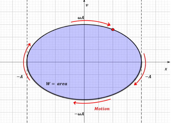
Figure 3: Phase-space diagram for Simple Harmonic Motion.
Let's note that Eq.(23) is a standard way of expressing an ellipse. It is well known that the area inside an ellipse can be expressed as \(W=\pi ab\) or, taking in our case \(a=A\) and \(b=\omega A\), we get \begin{equation}\tag{24} W = \pi \omega A^2. \end{equation}
Computation of average mechanical energy. In the case of SHM, the potential energy can be obtained from Hooke's Law: \(F = -kx\) and \(U = \frac{1}{2} kx^2\) and the kinetic energy is the same as before.
Consequently, due to the dependence on \(x\) and \(v\) concerning time, see Eq.(23), we can integrate them and yield the average kinetic and potential energies \begin{equation}\tag{25} \langle KE \rangle =\frac{1}{T}\int_{0}^{T}\frac{1}{2}mv^2dt = \frac{m\omega^2 A^2}{4}, \end{equation} \begin{equation}\tag{26} \langle U \rangle =\frac{1}{T}\int_{0}^{T}\frac{1}{2}kx^2dt = \frac{kA^2}{4}. \end{equation}
Now, the average mechanical energy for the simple harmonic motion can be expressed as \begin{equation}\tag{27} \langle E \rangle = \frac{m\omega^2 A^2}{4} + \frac{kA^2}{4}. \end{equation}
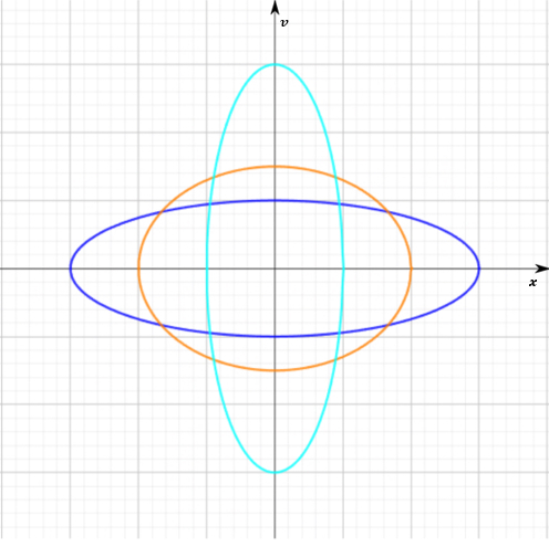
Figure 4: Variations in parameters \(\omega\) and \(A\) while maintaining \(W\) constant.
Optimization of energy. We can treat the amplitude \(A\) and the frequency \(\omega\) as free parameters and optimize the average energy (27) under the condition that the area (24) remains constant, see also Fig. 4.
By rearranging the area formula for amplitude, we can replace \(A^2\) with \(W/\pi \omega\) to simplify the average mechanical energy. \begin{equation}\tag{28} W = \pi A^2 \omega \rightarrow A^2= \frac{W}{\pi \omega}. \end{equation} \begin{equation}\tag{29} \langle E \rangle = \frac{m\omega^2 \frac{W}{\pi \omega}}{4} + \frac{k\frac{W}{\pi \omega}}{4} = \frac{m \omega W}{4\pi} + \frac{kW}{4\pi \omega}. \end{equation} Consequently, by optimizing the average mechanical energy, we can achieve the result. The first derivative: \begin{equation}\tag{30} \frac{d\langle E \rangle }{d\omega} = \frac{m W}{4\pi} - \frac{kW}{4\pi \omega^2} = 0. \end{equation} Solving this equation for the frequency \(\omega\), we get \begin{equation}\tag{31} \omega^2 = {\frac{k}{m}}. \end{equation} This means the actual periodic path the object takes under simple harmonic motion can be achieved under the condition that the square of angular frequency \(\omega^2\) corresponds to the spring constant over mass \(k/m\). The result obtained from Maupertuis's principle corresponds to the standard result obtained through simple harmonic motion standard equations.
The variational principle employed in quantum mechanics contrasts with Maupertuis's principle, which finds application in classical mechanics. However, the steps in their execution allow them to maintain an analogous relationship. Its execution can be broken down into the following steps:
1st Guess the behavior of the particle: it involves using adjustable parameters to develop a trial wave function that describes the system's quantum state. For example, a trial wavefunction may depend on regular space position \(x\) and on a free parameter \(a\) \begin{equation}\tag{32} \psi = \psi(x,a). \end{equation} Of course, for different systems the trial wavefunctions and parameters are different. Picking the form of the trial wavefunction is equivalent to picking the motion in Eqs.(6,23).
2nd Calculating the energy of the system: it requires calculating expectation values from the operators of kinetic and potential energies using the trial wavefunction from the first step: \begin{equation}\tag{33} E(a) = \langle \psi | \hat H | \psi \rangle = \int \psi^*(x,a) \,\hat H \,\psi(x,a) dx, \end{equation} where \(\hat H = \hat{KE} + \hat{U}\) is the Hamiltonian that represent the energy of the system. This step is equivalent to classical calculations of average mechanical energies (19,29).
3rd Optimization: usually numerical methods are used to optimize the parameters until the energy from step 2 value is minimized. If no other conditions are applied, the result approximates the ground state wavefunction and the ground state energy of the system (\(n=1\)) \begin{equation}\tag{34} \frac{d E}{d a} = 0. \end{equation}
| Similarities | Differences |
|---|---|
| Both require parametrization of the motion with a set of parameters. | The parameters for the variational principle rely on the Hamiltonian and wavefunction, while the Maupertuis's principle involves the phase-space diagram. |
| After the motion is defined, the energy can be minimized according to the parameters to be further optimized. | The optimization of energy with respect to the parameters results in the ground state of the wave function for the variational principle (state with certain quantum number), while for Maupertuis's principle minimization occurred for the fixed phase-space area. |
In summary, see Table 1, Maupertuis's and the variational principles share similarities in estimating motion, energy minimization, and optimization. They differ in the nature of the parameters and the outcomes of this process. Nevertheless, if analyzed based on their computational approach, they can be regarded as counterparts of different physical systems.
The paper aimed to expose Maupertuis's principle as an alternative approach to describe classical systems yielding standard equations and building a bridge with the variational principle implemented in quantum mechanics.
In conclusion, through the two cases explored, Maupertuis's principle resulted in Newton’s second law of motion, \( a = F/m, \) for scenarios with constant acceleration motion and for standard angular frequency equation, \( \omega^2 = k/m ,\) for the case resembling simple harmonic motion. The derivation of these well-known equations from an alternative approach, such as Maupertuis's principle, attests to its precision in describing dynamical systems. Moreover, when contrasted with the variational principle, they share similarities in their computational approaches; both require an estimation of motion under a set of parameters, and both involve minimization and optimization to complete their calculations. Despite these parallels, they diverge in the nature of their parameters and in their outcomes. While Maupertuis' principle yields a constant that aids in determining the actual path within a dynamical system, the variational principle is tailored for describing the wavefunctions of quantum states.
The author extends heartfelt thanks to the LaGuardia Honors program for their unwavering support, and to Dr. Roman Senkov for the insightful discussions and invaluable assistance.
[1] L.D. Landau, L.M. Lifshitz, "Mechanics: Volume 1". Butterworth-Heinemann, 1976.
[2] M. Spivak, "Physics for Mathematicians: Mechanics I". Publish and Perish, 2010.
[3] L.D. Landau, L.M. Lifshitz, "Quantum Mechanics: Non-Relativistic Theory". Butterworth-Heinemann, Jan. 1981.
[4] V. Zelevinsky, "Quantum Physics: Volume 1 - From Basics to Symmetries and Perturbations". Wiley, Dec. 2010.
[5] J.R. Taylor, "Classical Mechanics". University Science Books, 2005.
[6] A. Sommerfeld (1916). "Zur Quantentheorie der Spektrallinien". Annalen der Physik (in German). 51 (17): 1–94. https://zenodo.org/records/1424309.
[7] Wikipedia, Bohr-Sommerfeld Model. https://en.wikipedia.org/wiki/Bohr-Sommerfeld_model (as of March 2024).