
This work was done by LaGuardia students Daniel Gallego and Layla Xholi as a part of the Honors “General Physics I” class, Fall 2021. The project studies binary star systems and derives the corresponding Lagrange points.
The project was conducted under the supervision of Dr. Roman Senkov.
Other research projects done by students in the Physics Honors courses: “Orbital Decay of a Massive Black Hole”, “Computer Modelling of Physical Systems”, and “Atomic Nuclei and Pairing Correlations”.
Download this article: pdf (2.8Mb)
We studied Lagrange points and tried to locate them in any given binary star system. The obtained equations were applied to both a Sun-Earth-Moon scenario as well as a binary star system. Using Python we mapped the potential energy of various binary systems with different mass ratios and identified their respective Lagrange points. Today the Lagrange points of our Earth-Sun system are of special interests as the point furthest from the Sun, also known as \(L_2\), hosts NASA's newest and most powerful James Webb Telescope.
Video Credts: youtube channel Launch Pad Astronomy.
The planets in our solar system revolve around a single star, the Sun. The universe, however, is filled with stars that are orbiting other stars. We refer to these as binary star systems [1].
The technological advances made over the last century have enabled us to send rovers, telescopes and spaceships to places unimaginable before. Predicting the motions of all these objects in space requires a good understanding of complicated environments where multiple gravitational forces act.
In a two-body system, Kepler’s 3rd Law is sufficient to predict the motion of both objects. When a third body is introduced, the motion becomes more complicated since the objects are constantly pulled and pushed by multiple forces. In this project we analyze and describe motion in this intricate three-body problem.
To analyze a three-body system we present it as a binary system (for example, two stars orbiting the common center of mass or a star-planet system) and a third celestial body (for example, a planet or a moon). If we assume a third body of negligible mass, we can imagine that it will be of little to no consequence on the binary system's motion. Such examples exist and we can look at an Earth-Sun-satellite scenario.
Another simplification can be achieved by choosing a non-inertial frame of reference that is rotating together with the binary system. In this rotating frame the binary system will be stationary, so the third body will experience the gravitational forces from two stationary masses. Having a stationary binary system is very convenient, but the non-inertiality of the reference frame introduces an additional fictitious force that will contribute to the net force on the third body and to the potential energy of the entire system.
Using Python to create contour maps of the potential energy of our three-body system, we are able to locate its Lagrange Points often referred to as the “parking spots of space”. Those points, named after the mathematician of the same name, are interesting positions in space; any object placed at those points will experience the same orbital period as that of the binary-system.
It is possible to identify five Lagrange points in a given system of which two should be stable and three are unstable. Spacecraft and satellites positioned there need very little to no fuel to maintain their position. Today there are probes present at some of the Lagrange points of our Earth-Sun system and the point furthest from the Sun, also known as \(L_2\), is the home of NASA's newest and most powerful James Webb Telescope that was launched from French Guyana in December of 2021.
We will start by considering a two-body problem which corresponds to the motion of two stars about a common center of mass or motion of a planet in the gravitational field of a star.
According to the universal law of gravity, the gravitational force between two point-like masses is given by the following equation \begin{equation}\tag{1} \vec{F}= - G\frac{m_1 m_2}{r^2} \vec{n}, \end{equation} where \(m_1\) and \(m_2\) are the interacting masses, \(r\) is the distance between the masses, \(\vec{n}\) is the unit vector defining the direction of the force, and \(G=6.67\times10^{-11}\,Nm^2/kg^2\) is the universal gravitational constant.
It is also useful to define the potential energy of interaction of two point-like masses: \begin{equation}\tag{2} U(r)=-\int \vec{F}(r)\cdot d\vec{r} = -G\frac{m_1m_2}{r}. \end{equation} These two equations are common knowledge and have been used to analyze the two-body problem. If we introduce a third body, the motion of the binary system will not be affected assuming that we are considering a third body of negligible mass. This is often the case when looking at the relative mass of a planet compared to two much heavier stars, or a moon relative to a planet and a star. We can thus use the same equations.
Let us look at such system. We know that the two bodies, \(m_1\) and \(m_2\), will orbit the center of mass with a certain orbital speed. If we begin rotating with the system then \(m_1\) and \(m_2\) appear to become stationary. This “freezing” of the frame allows us to analyze more conveniently the motion and relationship between this binary system and the third body. This approach renders the frame non-inertial.
Traditionally, an inertial frame is required to apply Newton's laws of motion but for the sake of ease, we decide to use a rotating frame of reference. To preserve the laws of motion in this non-inertial frame we must introduce fictitious forces such as \(\vec{F} \rightarrow \vec{F} + \vec{F}_{NI}\). Such a fictitious force acting on the third body can be written as \begin{equation}\tag{3} \vec{F}_{NI} = m \omega^2 \vec{r}, \end{equation} where \(m\) is the mass of the third body, \(\omega\) is the angular velocity of the binary system, and \(\vec{r}\) is the position of the third body relative to the center of the binary system [2]. The corresponding potential energy that can provide this fictitious force is given by \begin{equation}\tag{4} U_{NI} = -\int \vec{F}_{NI}(r)\cdot d\vec{r} = - \frac{1}{2} m \omega^2 r^2. \end{equation}
Now let's consider a three body system and write the equation for the corresponding Lagrange points. In the rotating frame, at any Lagrange point all the forces acting on the third-body balance out each other, so the third body is stationary relative to the binary system. The corresponding equation can be written as \begin{equation}\tag{5} \vec{F}_{1}+\vec{F}_{2}+\vec{F}_{NI}=0, \end{equation} where \(\vec{F}_{1}\) is the force between one component of the binary system and the third body, \(\vec{F}_{2}\) is the force between the second component of the binary system and the third body, and \(\vec{F}_{NI}\) is the fictitious force on the third body due to non-inertiality of the frame.
Another way to determine Lagrange points is to find local extrema of the potential energy of the third body in the binary system field \begin{equation}\tag{6} \delta U(r) = 0, \end{equation} where \(U(r) = U_{1}(r) + U_2(r) + U_{NI}(r)\) is the energy of interaction of the third body with \(m_1\), \(m_2\), and the fictitious (so called centrifugal) potential energy. Equations (5) and (6) are equivalent.
In this section we apply the above equations to the Sun-Earth system and analytically solve for the simplest Lagrange Points located near the Earth. We consider the situation represented on Fig. 1.
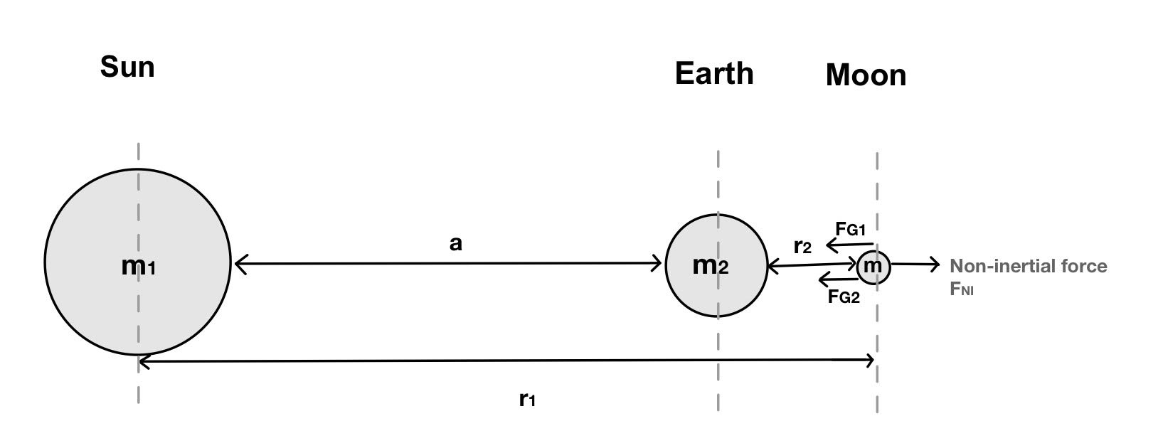
Figure 1: Graphical representation of the forces present in a three-body system.
Using universal law of gravity (1) and the non-inertial force (3) we can rewrite Eq.(5) as \begin{equation}\tag{7} -G\frac{m_1 m}{r_1^2}-G\frac{m_2 m}{r_2^2}+ m \omega^2 r_3 = 0, \end{equation} where \(r_1\) is the distance from the Sun to the mass \(m\), \(r_2\) is the distance from the Earth to the mass \(m\), \(r_3 \approx r_1\) is the distance from mass \(m\) to the center of the Sun-Earth system, and \(\omega\) it's angular velocity of the Sun-Earth system. Here we assumed that the Sun is much more massive than the Earth, \(m_2 \gg m_1\).
Using Kepler's third law we can find the angular velocity \(\omega\) as \begin{equation}\tag{8} \omega^2 \approx G\frac{m_1}{a^3}, \end{equation} where \(m_1\) is the solar mass and \(a\) is the average radius of Earth's orbit, so called Astronomical Unit or AU. Now we can rewrite the balance of forces (7) as \begin{equation}\tag{9} G\frac{m_1 m}{r_1^2} +G\frac{m_2 m}{r_2^2} = G\frac{m_1}{a^3} m r_1. \end{equation} It is convenient to divide by \(G m_1 m\) on both sides of Eq. (9) and introducing the ratio \begin{equation}\tag{10} \mu = \frac{m_2}{m_1}, \end{equation} we finally get \begin{equation}\tag{11} \frac{1}{r_1^2}+\frac{\mu}{r_2^2}= \frac{r_1}{a^3}. \end{equation} We can measure all the distances in AU so that \(a = 1\) and \begin{equation}\tag{12} \frac{1}{r_1^2}+\frac{\mu}{r_2^2}= r_1. \end{equation}
To solve Eq.(12) we will substitute \begin{equation}\tag{13} r_1 = 1 + \delta r\, \mbox{ and }\, r_2 = \delta r, \end{equation} where \(\delta r \ll 1\) is the deviation of \(r_1\) from 1 AU. Using the smallness of \(\delta r\) and applying Taylor expansion [3], \begin{equation}\tag{14} \frac{1}{(1+\delta r)^2} \approx 1 - 2 \delta r, \end{equation} we finally arrive at \begin{equation}\tag{15} 1 -2\delta r + \frac{\mu}{\delta r^2} \approx 1 + \delta r. \end{equation}
The method works best by choosing a point far enough into the series to grant a good approximation and then “cutting of” the tail of the polynomial chain there. Following this principle we obtain: \begin{equation}\tag{16} \delta r = \left(\frac{\mu}{3} \right)^{1/3}. \end{equation}
This allowed us to find the \(L_2\) point for our Earth-Sun system. For the Sun-Earth system \(\mu = 1/330000\) and Eq.(16) gives \(\delta r =0.01\) AU.
We were then able to calculate for the other point \(L_1\) located on the other side of the Earth also at 0.01 AU. To do so we simply had to subtract \(\delta r\) instead of adding it an change the corresponding sign in Eq.(7) because of the different direction of the force.
Now let us consider an arbitrary three-body system. Instead of using forces to look for the precise location of each Lagrange point, we use potential energy, denoted as \(U\), to visualize the extrema. Those extrema would represent our Lagrange points. Using potential energy is much easier to deal with than forces because it's not a vector. Finding the potential energy extrema is equivalent to what is done in Eq (5) where we set the forces equal to zero.
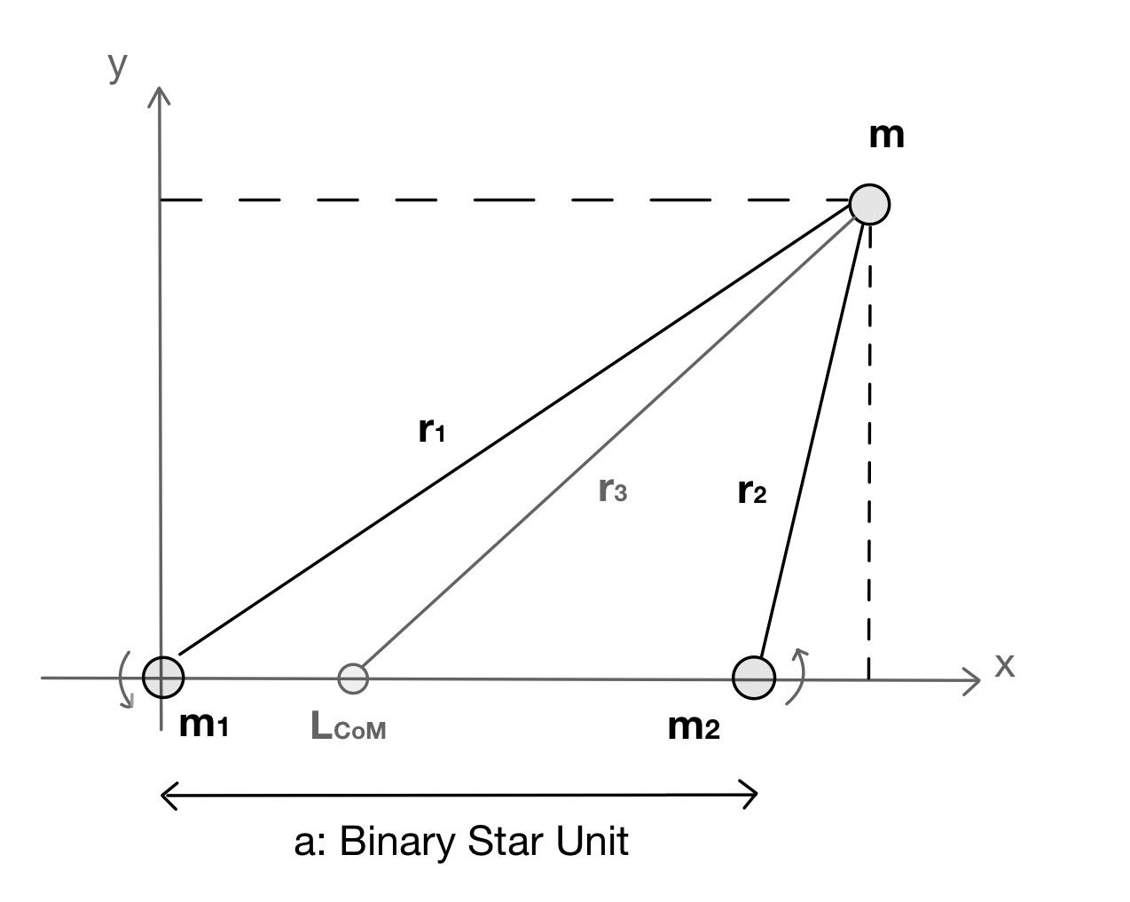
Figure 2: Chart of binary star system showing center of mass, as used in mapping potential energies of different binary systems based on different masses, in BSU.
Figure 2 can then be utilized to introduce the center of mass for any arbitrary binary system with different distances from a mass of interest. With this we can derive the parameters of this three-body system that we wish to use later. If the coordinates of mass \(m\) are \( (x,y)\), then \begin{equation}\tag{17} r_1= \sqrt{x^2+y^2}, r_2= \sqrt{(x-a)^2+y^2}, r_3=\sqrt{(x-l)^2+y^2}, \end{equation} and center of mass position \(l\) and the angular velocity \(\omega\) are \begin{equation}\tag{18} l=\frac{m_2}{m_1+m_2}a ,\; \omega^2 = \frac{G(m_1+m_2)}{a^3}, \end{equation} where \(a\) is the size of the binary system and the angular velocity \(\omega\) is expressed in terms of \(G\), the total mass \(m_1+m_2\), and the size \(a\). Using the above parameters we can piece together an equation for potential energy of the system as follows: \begin{equation}\tag{19} U(x,y) = - \frac{Gm_1 m}{r_1} - \frac{Gm_2 m}{r_2} - \frac{m\omega^2 r_3^2}{2}, \end{equation} which corresponds to the following after substituting all the appropriate parameters: \begin{equation}\tag{20} U(x,y) = - \frac{Gm_1m}{\sqrt{x^2 + y^2}} - \frac{Gm_2m}{\sqrt{(x-a)^2 + y^2}} -\frac{G(m_1+m_2)m}{2a^3} \left((x-l)^2+y^2\right). \end{equation}
To make the equation more manageable we try to simplify components of the equation. It is convenient to divide Eq.(20) by the 'typical' potential energy \(G(m_1+m_2)m/a\) and introduce ratio of each mass to the total mass as \begin{equation}\tag{21} \mu_1 = \frac{m_1}{m_1+m_2},\; \mu_2 = \frac{m_2}{m_1+m_2},\; \mbox{ and } \mu_1 + \mu_2 = 1, \end{equation} and measure all the distances in the size of the binary system \(a\) \begin{equation}\tag{22} r_1 \rightarrow a r_1,\; r_2 \rightarrow a r_2,\; r_3 \rightarrow a r_3. \end{equation} Now the 'reduced' potential energy \( u = U/[G(m_1+m_2)m/a] \) looks like: \begin{equation}\tag{23} u(x,y) = - \frac{\mu_1}{r_1} - \frac{\mu_2}{r_2}-\frac{ r_3^2 }{2}, \end{equation} where \(r_1 = \sqrt{x^2+y^2}\), \(r_2 = \sqrt{(x-1)^2+y^2}\), and \({r_3} = \sqrt{(x-\mu_2)^2+y^2}\).
Using the end result, Eq (23) allows us to change the parameters \((\mu_1, \mu_2)\) quite easily in a program we wrote in Python to show the results for very different types of binary systems. We were able to use the same equation for our Sun-Earth-Moon system, and for binary system with different mass distribution ratios. Potential energy diagrams were mapped for binary star systems of nearly equal mass as well as systems with a ratio of 80:20.
Though motion in three-body systems are complicated it is possible to analyze them under certain assumptions. Computational tools can help us map the potential energy of such systems and locate Lagrange points.
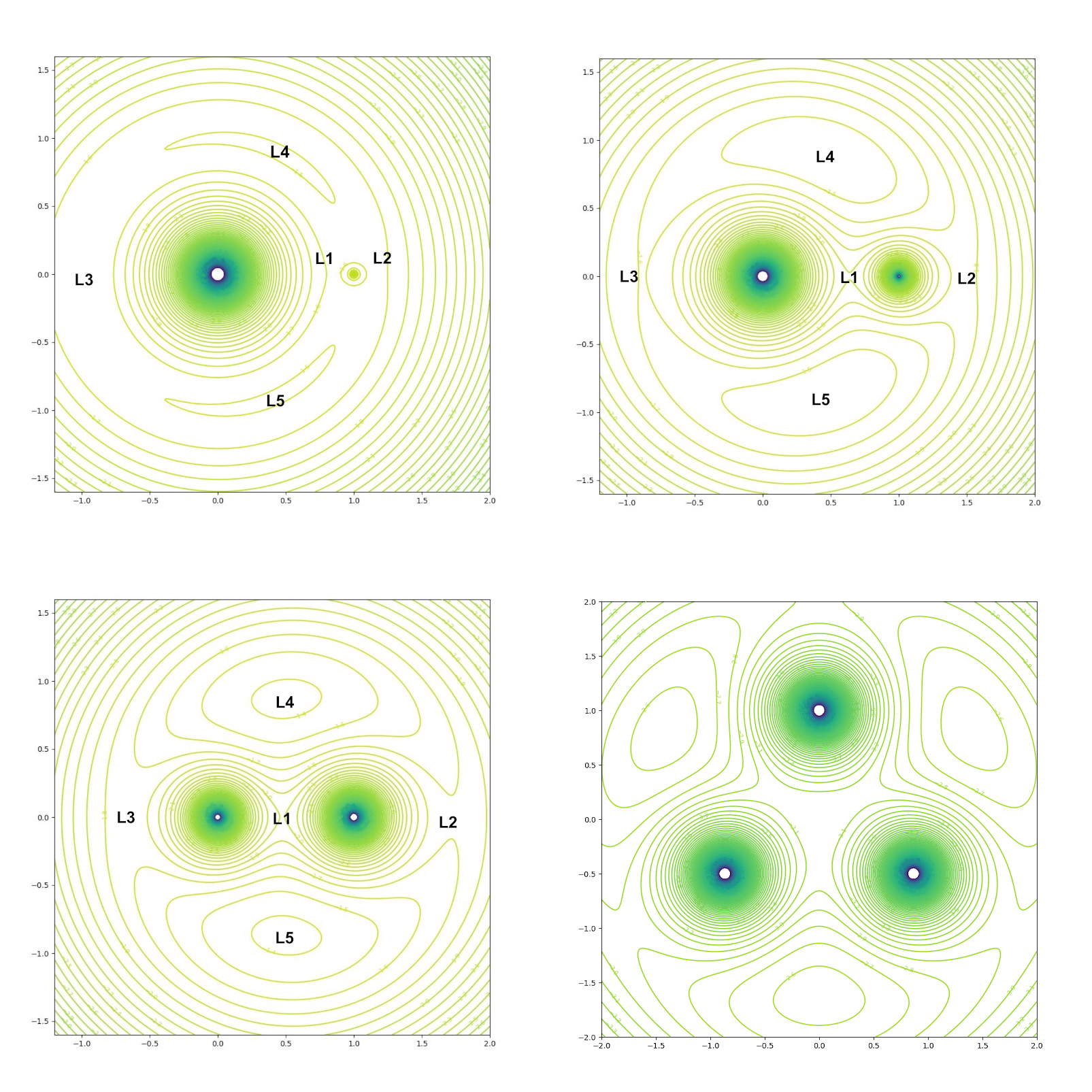
Figure 3: Top left: PE diagram depicting the five Lagrange Points in our Earth-Sun-system. Top right: PE diagram for a system with a smaller difference in masses between the two bodies. The mass difference here is 80 to 20. Bottom left: PE diagram for a recently discovered binary system in the NGC 1850 cluster [4]. The binary system is composed of a main sequence turn-off star and a black hole with a mass ratio of 5 to 11. Bottom right: PE diagram for a system composed of three stars of equal mass.
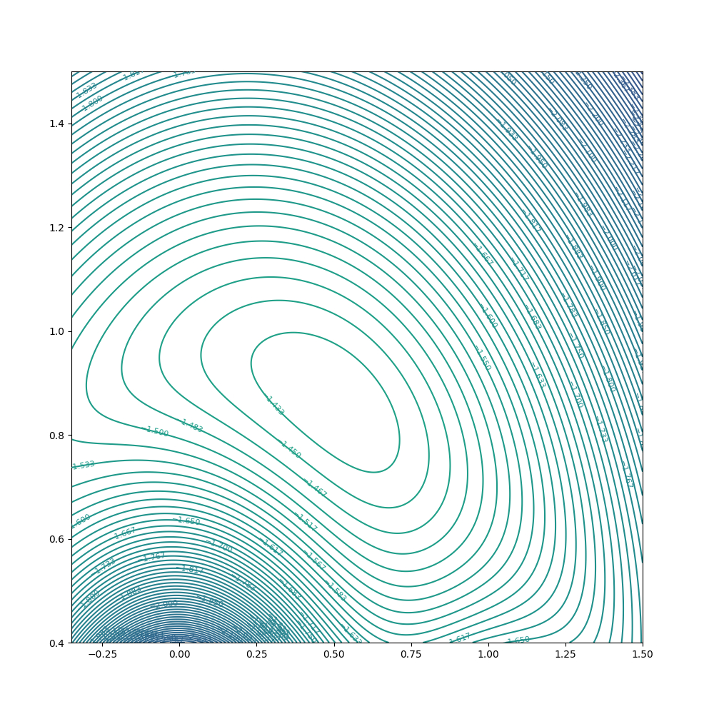
Figure 4: A closer look at a Lagrange point on a potential energy diagram. Here a stable point is depicted, which corresponds to a minimum peak.
The resulting potential energy contour maps, Figures 3, 4 and 5, show that a binary system's Lagrange points are affected by the mass distribution of the two bodies \(m_1\) and \(m_2\), as predicted. Interestingly the \(L_1\) point, the point between both masses, appears to be the same between most types of binary systems. The stable Lagrange points, \(L_4\) and \(L_5\), appear to decrease in size as the disparity between \(m_1\) and \(m_2\) becomes more significant. A system with a mass ratio of about 80:20 shows these stable points to be larger, meaning there could be a wide deviation in the movement of an object there before it leaves equilibrium.
Figure 5: An animation demonstrating evolution of the potential energy field and the corresponding Lagrange points of a binary system. The binary system mass distribution changes from \( \mu_1 = 0.9, \mu_2 = 0.1\) to \( \mu_1 = 0.1, \mu_2=0.9\).
While human space exploration has its limits, it is not unreasonable to imagine sending satellites, telescopes and probes to occupy these points in space.
The authors would like to thank Dr. Roman Senkov for his help and guidance in this research project. The research was done as a part of the Honors General Physics I course at LaGuardia Community College.
[1] S. Naimi et al., Phys. Rev. C 86, 014325 (2012).
[2] https://en.wikipedia.org/wiki/Fictitious_force
[3] https://web.ma.utexas.edu/users/m408s/CurrentWeb/LM11-11-2.php