
by Liting Zheng, Seungyeon Lee, Ling Lin, and Jun Hong (LaGuardia CC, Computer Science, 2022-2024 CRSP cohorts)
The work was done as a part of the CRSP program at LaGuardia Community College/CUNY, under the supervision of Dr. Yun Ye and Dr. Shenglan Yuan.
This article has been published as part of the Special Edition of Ad Astra, which features the CUNY Research Scholars Program (CRSP) across The City University of New York. The issue is accessible at http://www.adastraletter.com/2024/crsp-special-edition/.
ABOUT THE AUTHORS
Jun Hong
Jun Hong, a Computer Science student at CUNY LaGuardia Community College plans to graduate in the Spring of 2024. He aspires to further his academic journey by transferring to a four-year institution. He has been working with Professor Yun Ye and Professor Shenglan Yuan since Fall 2023, and is very excited for what the future holds as he continues his studies.

Seungyeon Lee
Seungyeon Lee, a Computer Science graduate from LaGuardia Community College and currently enrolled at Hunter College, has been actively engaged in research projects under the guidance of Dr. Yun Ye and Dr. Shenglan Yuan since LaGuardia.

Ling Lin
Ling Lin is a Computer Science student at LaGuardia Community College. After she graduates from LaGuardia, she plans to transfer to a four-year university to delve into the field of Computer Science. With the mentorship of both Dr. Yun Ye and Dr. Shenglan Yuan, she has gained insight into both hardware and software algorithm implementation.

Liting Zheng
Liting Zheng is a Computer Science student at LaGuardia Community College, and she plans to pursue a bachelor's degree at a four-year college after earning her associate's degree. She is currently working on underwater acoustic communication and hardware implementation under the supervision of Dr. Yun Ye and Dr. Shenglan Yuan with the support of CRSP.
This paper focuses on the efforts of our team to develop an embedded hardware platform for underwater acoustic communication that can handle changing environmental conditions and also support high data rates. We implemented a basic wireless communication system design, microcomputer architecture, and hardware interfacing using the Digilent Eclypse Z7 board. We then employed algorithms such as the Mean Squared Error (MSE) and Least Mean Square (LMS) to process and analyze the data received from our experiments. While the process of discovering the most accurate ratios and coefficients needed for the algorithms is still ongoing, the results of the transmitter and receiver tests show that changes in distance, depth, and frequency have a significant impact on the signals detected by the hydrophones, which illustrates the system’s capability to respond to diverse environmental parameters.
Underwater acoustic communication (UAC) is a system used to transmit and receive messages under water; it is essential for many industries, such as commercial, scientific, meteorology, agricultural, military, and much more. From scuba divers signaling one another, submarines navigating the depths of the sea, to tsunami warning detection, UAC is a necessity.
To understand UAC systems, the research consists of two parts: set up an embedded hardware platform to test the communication between a transmitter and receiver underwater; then implement the Mean Squared Error (MSE) and Least Mean Square (LMS) algorithms to analyze the results and pinpoint the most accurate values. For the hardware platform, our team used the Digilent Eclypse Z7: Zynq-7000 SoC Development Board. Its main purpose is to “enable the rapid prototyping and development of embedded measurement systems” [3]. The software used by the Eclypse Z7 is Vivado Design Suite by Xilinx, which is a special software for the design and analysis of hardware description language (HDL) – a computer language for hardware that differs from more common programming languages like Java or C++.
The procedure for the experiment involves the Eclypse Z7 board in conjunction with transceiver hydrophones and other devices which contain a digital-to-analog converter. The transmitter emits acoustic signals, and the receiver captures and stores the signals with an analog-to-digital converter. The data obtained from experiments are analyzed by two algorithms – the Mean Squared Error (MSE) and Least Mean Square (LMS) along with MATLAB, a programming and numerical computing platform. Comparing both the MSE and LMS algorithms, our team is able to process our data to obtain the utmost accurate values [4].
Due to the increase of communication systems including 5G networks and more, the demand for underwater acoustic communication’s expansion is increasing at an unprecedented rate. This research provides an effective demonstration of underwater acoustic communication by developing an adaptable embedded hardware platform, receiving data, and using algorithms to analyze and process this data.
The Digilent software is installed on a micro-SD card, which is then connected with the Eclypse board to verify connection with Xilinx software. The transmitter is then linked to the DAC board interface of the Digilent Eclypse Z7, which plays a pivotal role in signal transmission. Prior to transmission, a human voice is recorded and modulated in three different frequencies. This modulated signal is fed into the DAC, which converts the digital representation of the voice signal into an analog form suitable for transmission.
To ensure optimal signal strength, the analog signal is amplified and connected to the DAC board interface. Then this amplified analog signal is transmitted underwater via an underwater speaker. The transmitted signals are captured by a hydrophone. These analog signals are routed through an analog front end circuit. The ADC interface on the Eclypse Z7 board converts these received analog signals into their digital counterparts [3]. In the experiment, various distances and depths of the receiver and transmitter underwater are used to study the performance of the communication systems. The results reveal whether different distances, depths, and modulations affect the received signals detected by the hydrophone.
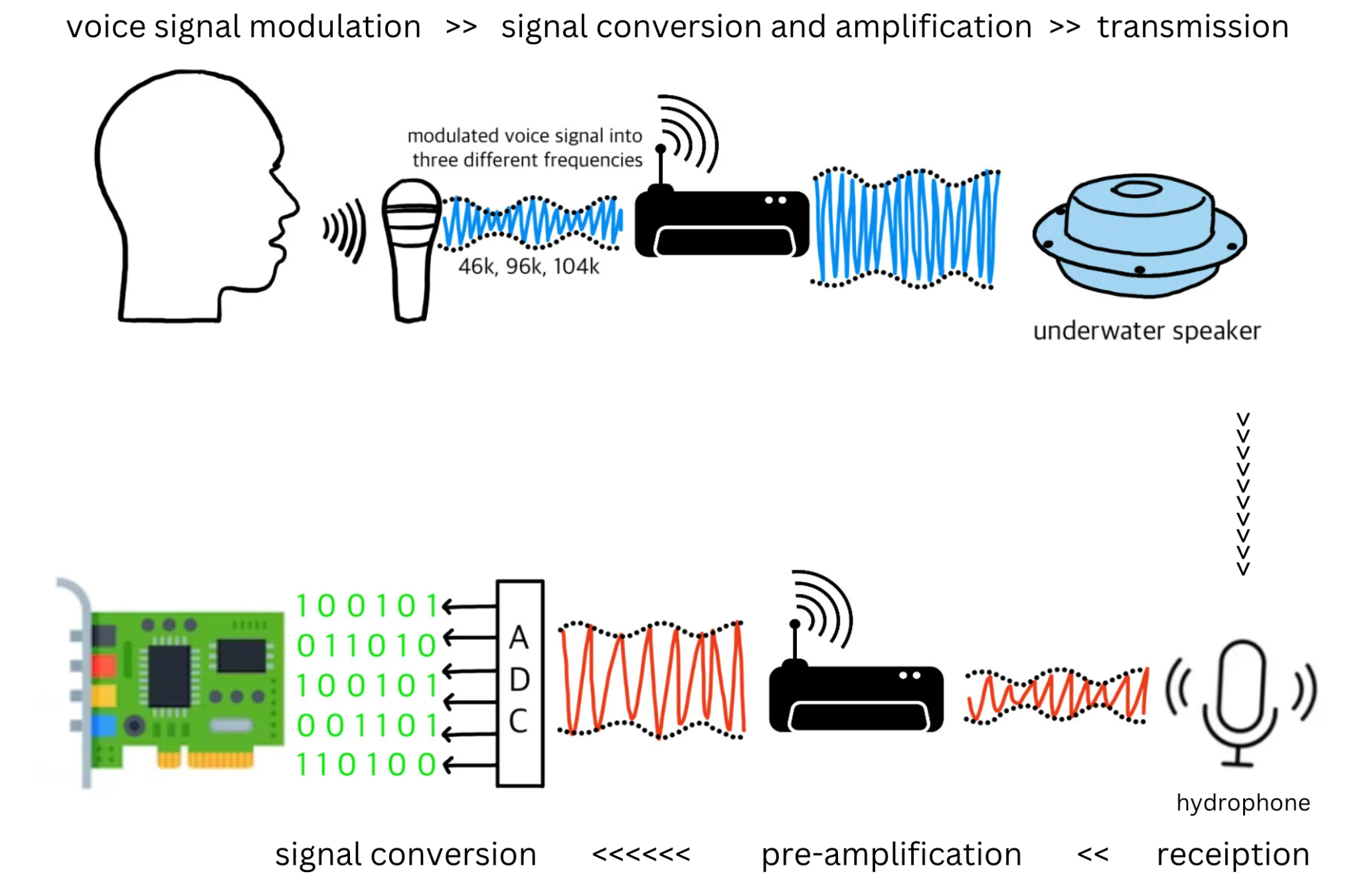
Figure 1: Underwater Communication System Setup.
Our next goal is to construct a software environment on the host laptop so that the microcomputer and host laptop can communicate successfully. To achieve the goal, we begin by downloading and installing the “Vivado Xilinx SDK 2019.1” on the Ubuntu 18.04.4 LTS operating system. Subsequently, to create a complete SDK workspace and execute the project on the Linux platform, we download and import the Zmod library from the Digilent website and add the SYSROOT Environment Variable within the SDK [2]. By doing this, we provide a development platform for using Digilent Zmods, while also ensuring that the build process can correctly locate the root file system. Furthermore, we install the PuTTY software to find the IP address of Eclypse Z7, connect a router to both the host laptop and the Eclypse Z7, and input the obtained IP address into the “Target Connections” within the Xilinx SDK. With these steps, we are able to compile and execute the project on the hardware board.
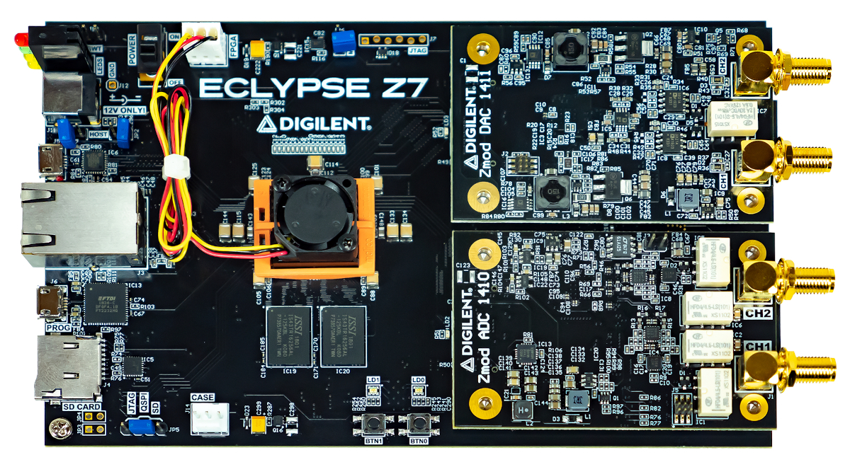
Figure 2: Eclypse Z7 board [3].
1. Mean Squared Error (MSE) Method
The idea of Mean Squared Error has existed for a long time and is widely used in the field of statistics and signal processing. It is an effective method to quantify the difference between actual values and predicted values. To evaluate the performance of the collected signal data, we apply MSE to analyze the received and original signals \begin{equation}\tag{1} \mbox{MSE} = \frac{\sum_i(y_i-p_i)^2}{n}, \end{equation} where \(y_i\) is original signal values, \(p_i\) is received signal values, and \(n\) is the total number of data [6]. When the original signal value matches the received signal value perfectly, the MSE will be zero. A larger MSE value means a poorer performance of the received signal [6].
To process and analyze signals, we start with resampling the original signal to match the sampling rate of the received signal. Next, we apply the Fast Fourier Transform (FFT) to transform the data from the time domain to the frequency domain. To further assess the performance of received signals in the frequency domain, instead of comparing the entire received signal with the resampled original signal directly, we apply a sliding window technique. This technique segments the received signal into portions and ensures each segment matches the duration of the original signal. Lastly, we apply the MSE method to compare the difference between each selected portion and the original signal. This process iterates and shifts by one sample at each step until all the received data has been examined.
After comparing the original signal with received signals under different range and depth conditions, we discover that the received signal has the best performance when the range is 1 meter and the depth is 1.524 meters as shown by Table1.
Table 1 below shows the theoretical and simulation results of stress and displacement for an aluminum cantilever beam subjected to a 44.42N force at the free end at various temperatures.
| Range | Depth | MSE | Ave. of MSE |
|---|---|---|---|
| 1m | 0 m | 0.03837 | 0.036594 |
| 0.762 m | 0.03952 | ||
| 1.524 m | 0.03189 | ||
| 2m | 0 m | 0.03832 | 0.038785 |
| 0.762 m | 0.03876 | ||
| 1.524 m | 0.03927 | ||
| 5m | 0 m | 0.03821 | 0.03853 |
| 0.762 m | 0.04192 | ||
| 1.524 m | 0.03547 |
2. Adaptive Least Mean Square (LMS) Algorithm
In acoustic research and application areas dealing with imprecisely known or variable conditions, a method to accommodate uncertainty or change is necessary. The LMS algorithm is a widely used adaptive filtering algorithm in digital signal processing. It updates the coefficients of a filter to minimize the mean square error between the desired and actual output. The simplicity, computational speed, and robustness of LMS enables optimal performance in systems over time-varying input signals, providing real-time processing and adaptation to changing environments [5].
For simplicity, we use two taps to illustrate how the adaptive LMS algorithm works as shown in Eq.(2) below. We will update the weight of the taps to minimize the sum of squared errors after continuing to analyze the transmitted and received data. \begin{equation}\tag{2} h_n(i+1) = h_n(i) + \mu e(i) X_n(i+1), \end{equation} here \(h_n(i)\) is the value of the n-th coefficient at sampled data \(i\), \(\mu\) is the step size learning rate, \(e(i)\) is the error signal at \(i\), and \(X(i)\) is the input signal at sampled data \(i\) corresponding to the n-th coefficient.
Audio recordings were loaded to represent the transmitted signals \([X(i-1),X(i),X(i+1)]\) and received signals \([Y(i),Y(i+1)]\) as in \begin{equation}\tag{3} \left[\begin{array}{l} \hat Y(i) \\ \hat Y(i+1) \end{array} \right] = \left[\begin{array}{lll} h_0(i) & h_1(i) & 0 \\ 0 & h_0(i) & h_1(i) \end{array} \right] \cdot \left[\begin{array}{l} X(i-1) \\ X(i) \\ X(i+1) \end{array} \right], \end{equation} \begin{equation}\tag{4} \left[\begin{array}{l} e(i) \\ e(i+1) \end{array} \right] = \left[\begin{array}{l} Y(i) \\ Y(i+1) \end{array} \right] - \left[\begin{array}{l} \hat Y(i) \\ \hat Y(i+1) \end{array} \right], \end{equation} \begin{equation}\tag{5} \left[\begin{array}{l} h_0(i+1) \\ h_1(i+1) \end{array} \right] = \left[\begin{array}{l} h_0(i) \\ h_1(i) \end{array} \right] + \frac{1}{2} \cdot \left[\begin{array}{lll} e(i) & e(i+1) & 0 \\ 0 & e(i) & e(i+1) \end{array} \right] \cdot \left[\begin{array}{l} X(i) \\ X(i+1) \\ X(i+2) \end{array} \right], \end{equation} where \(i\) starts at 1. The initial two tap weights \([h_0(i),h_1(i)]\) are then adapted based on updated transmitted and received signals. These coefficients are used to predict the received signals \([\hat Y(i),\hat Y(i+1)]\) and calculate the difference \([e(i),e(i+1)]\) between the predicted values and the actual received values, so that the sum of the square of errors will be minimized. Simply put, to reach the optimal number of tap weights, the new tap weight is based on the previous tap weight plus the proportional value of \(e(n)X(n)\) (depicted as the matrices and in Eq.(2)) [5].
The updated coefficients are computed \([h_0(i+1),h_1(i+1)]\) by using the previous \([h_0(i),h_1(i)]\) coefficients, \( e(i), e(i+1)\) errors, \(X(i-1), X(i), X(i+1)\) transmitted signals, and a constant \(\mu\) (for now we chose 0.5, but we will test other constants) to iteratively determine the next set of coefficients until all the signal data has been processed.
There are many different steps in our process of developing an embedded hardware system for underwater acoustic communication. Everything must be accurate due to the importance of communication and efficient due to hardware limitations. The final step in the hardware configuration is to complete the Eclypse Z7 setup. After that, we can conduct the experiment and analyze our own data using the MSE and LMS algorithms.
The end goal for using the algorithms to process our data is to find the optimal amount of taps to use and minimize our error between the actual y- and predicted y- values, because the errors (e) should converge to 0 as the amount of iterations (n) increases.
The reason for using the LMS over the MSE algorithm was due to the LMS being an adaptive filter - it adjusts its values depending on the previous set of data [4]. Also, with the LMS we can increase the number of taps - the MSE only uses 1 tap and our next steps are to try the LMS with multiple taps and find the right balance. If too little taps are used, the results may be inaccurate. If too many taps are used, we lose efficiency. We also need to find the best constant to converge towards 0 quicker- as of now we used 0.5 as a starting point but that is not necessarily the best choice.
We also have 9 different audio recordings based on receiving distance (from 1m to 5m), and so far we’ve only been analyzing two of them.
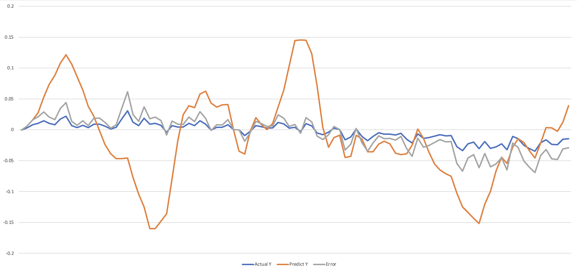
Figure 3: A graph depicting the errors, predicted y-values, and actual y-values.
In Figure 3 we see that our errors have not yet converged to 0, and that is an issue that occurs due to incorrect tap lengths, the wrong value for step size \(\mu\), or both. We will deduce the most efficient number of taps and parameters that give us the most accurate results. Currently, our research has only been focused on analyzing the results of the data using the time domain, because the LMS is originally used as an adaptive filter for the time domain. We can increase accuracy of our results by also analyzing the frequency domain, which we will do in the future. Our goals are to complete the hardware configuration and find the most accurate parameters in the LMS to end up with the most precise results.
[1] “Adaptive Filter - an Overview | ScienceDirect Topics.” www.sciencedirect.com, https://www.sciencedirect.com/topics/engineering/adaptive-filter, Accessed 8 Feb. 2024.
[2] “Digilent/Zmodlib.” GitHub, 22 Aug. 2023. github.com/Digilent/zmodlib. Accessed 8 Feb. 2024.
[3] “Eclypse Z7: Zynq-7000 SoC Development Board with SYZYGY-Compatible Expansion.” Digilent. digilent.com/shop/eclypse-z7-zynq-7000-soc-development-board-with-syzygy-compatible-expansion/.
[4] “Introduction to Least Mean Square Algorithm with MATLAB.” Hardwareteams.com, https://hardwareteams.com/docs/dsp/lms-algorithm/, Accessed 8 Feb. 2024.
[5] Farhang-Boroujeny, Behrouz. (2013). Adaptive Filters: Theory and Applications (2nd Edition). (pp. 139-173). John Wiley & Sons, Ltd.
[6] “Mean Squared Error (MSE).” Statistics by Jim, https://statisticsbyjim.com/regression/mean-squared-error-mse/, Accessed 9 Feb. 2024.